After a brief stint with several interesting computer vision projects, include this and this, I’ve recently decided to take a break from computer vision and explore reinforcement learning, another exciting field. Similar to computer vision, the field of reinforcement learning has experienced several important breakthroughs made possible by the deep learning revolution. AlphaGo, a GO playing AI trained by reinforcement learning, became the first computer program to surpass human in the game of GO. If you think this is not impressive enough, in July this year, a team from OpenAI used reinforcement learning to train an AI that beats the world champion human player in DOTA 2. All of these were not possible if not for the recent advancement of reinforcement learning and deep learning.

So what exactly is reinforcement learning?

In short, the objective of reinforcement learning is to train an intelligent agent that is capable of interacting with an environment intelligently. For instance, in the game of Go, the GO playing AI learns to excel in playing the game (the environment) through playing tens of thousands of game over and over again (usually with itself!) and discovers subtle strategies through trial and error. At present, the two most popular classes of reinforcement learning algorithms are Q Learning and Policy Gradients. Q learning is a type of value iteration method aims at approximating the Q function, while Policy Gradients is a method to directly optimize in the action space.

In this article, I will outline the pros and cons of each method and test them on the VizDoom environment (see below for a description). In all of our experiments, the agents will only learn from raw pixel inputs with no knowledge of the game internals such as the map of the environment and the coordinates of the enemies.

VizDoom Environment

There are several scenarios that come with VizDoom. I choose the Defend the Center scenario since it provides a challenging 3D partially observable environment yet not too hard such that reinforcement learning will fail to find a good solution. Below is a screenshot of what the scenario looks like.

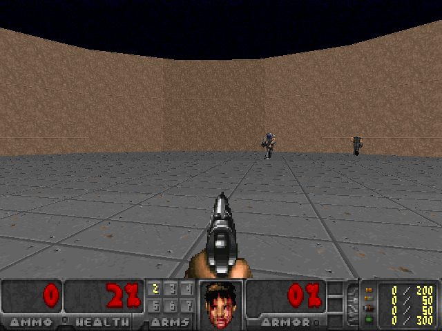
In this scenario, the agent occupies the center of a circular arena. Enemies continuously got spawned from far away and gradually move closer to the agent until they are close enough to attack from close range. The agent is equipped with a handgun. With limited bullets (26 in total) and health, its objective is to eliminate as many enemies as possible while avoid being attacked and killed. By default, a death penalty of -1 is provided by the environment. In order to facilitate learning, I enriched the variety of rewards (reward shaping) to include a +1 reward for every kill, and a -0.1 reward for losing ammo and health. I find such reward engineering trick to be quite crucial to get the agent to learn good policies.

Q Learning and DQN

Q Learning is a traditional reinforcement learning algorithm first introduced in 1989 by Walkins. It is a widely used off the shelf method that is usually used as baseline for benchmarking reinforcement learning experiments. For those of you just started out with reinforcement learning who are not familiar with Q Learning and DQN, I strongly recommend you to read this great article.

Here is a high level description of what Q Learning is. To reiterate, our goal is to train an agent who is capable of interacting with an environment intelligently. In the beginning, our agent knows nothing about the environment. Each time the agent interacts with the environment, we obtain a data point <\(s\),\(a\),\(r\),\(s^\prime\)>, where \(s\) represents the state, which is an observation from the environment, \(a\) is the action the agent takes, \(r\) is the reward given by the environment to tell how “good” the action is, and \(s^\prime\) is the next state after transitioning through the environment. Q Learning is an algorithm to approximate the Q function through learning from the stream of <\(s\),\(a\),\(r\),\(s^\prime\)> data points. First of all, we have to define Q function. Q function is the expected value of the sum of future rewards by following policy \(\pi\)

You can think of policy \(\pi\) as a strategy book to instruct the agent what actions to take at any given states. \(R_t\) represents the sum of discounted future rewards.

The idea of Q Learning is that if we have a good approximate of Q function for all state and action pairs, we can obtain the optimal policy \(\pi^*\) by the following expression

But how can we make use of the data points <\(s\),\(a\),\(r\),\(s^\prime\)> to approximate Q? This is where Q Learning comes in. It turns out that there is this neat equation called the Bellman equation that relates the Q functions of consecutive time steps

We can then use this Bellman equation to iteratively approximate the Q function through temporal difference learning. Specially, at each time step, we seek to minimize the the mean squared error of the \(Q(s,a)\) (prediction term) and \(r + \gamma\max_{a^\prime} Q(s^\prime,a^\prime)\) (target term)

In practice, we usually use a deep neural network as the Q function approximator and apply gradient descent to minimize the objective function \(L\). This is known as Deep Q Learning (DQN). A close variant called Double DQN (DDQN) basically uses 2 neural networks to perform the Bellman iteration, one for generating the prediction term and the other for generating the target term. This will help alleviate bias introduced by the inaccuracies of Q network at the beginning phase of training.

This pretty much summaries Q Learning and DQN. Let’s talk about Policy Gradients.

Policy Gradients

While the goal of Q Learning is to approximate the Q function and use it to infer the optimal policy \(\pi^*\) (i.e. \(arg\!\max_a Q(s,a)\)), Policy Gradients (PG) seeks to directly optimizes in the policy space. What do we mean by that? In Policy Gradients, we usually use a neural network (or other function approximators) to directly model the action probabilities. Each time the agent interacts with the environment (hence generating a data point <\(s\),\(a\),\(r\),\(s^\prime\)>), we tweak the parameters \(\theta\) of the neural network so that “good” actions will be sampled more likely in the future. We repeat this process until the policy network converge to the optimal policy \(\pi^*\).

Formally, the objective of Policy Gradients is to maximize the total future expected rewards \(E[R_t]\), where \(R_t\) represents the sum of future discounted rewards. We want to iteratively tweak the parameters \(\theta\) of our policy network so that \(E[R_t]\) is maximized. How can we achieve that? This is where Policy Gradients comes in. It turns out that there is this nice formula for the gradient of \(E[R_t]\)

Using this above expression to approximate the gradient of \(E[R_t]\) is called REINFORCE. Intuitively, \(R_t\) is the scaling factor which dictates how the \(P(a)\) should change in order to maximize the expected future rewards. If action \(a\) is good (i.e. large \(R_t\)), \(P(a)\) will get pushed up by a large magnitude, on the other hand, if action \(a\) is bad (i.e. small or negative \(R_t\)), \(P(a)\) will be discouraged. Eventually, good actions will have an increased likelihood to get sampled in future iterations. The above formulation is often known as the Actor-Critic framework, where the policy network acts as the “Actor” (i.e. sample actions) and \(R_t\) acts as the “Critic” to evaluate the “goodness” of the sampled actions.

Similar to Q Learning, we can use the stream of <\(s\),\(a\),\(r\),\(s^\prime\)> sampled data points to estimate the gradient of \(E[R_t]\), and apply gradient ascent to maximize \(E[R_t]\). For more information on Policy Gradients and the derivative of the Policy Gradients formula above, I strongly recommend this blog post written by Karpathy.

Now we have a basic understanding of Q Learning and Policy Gradients. So the natural question is how do they stack up against each other? On what occasions should we use Policy Gradients over Q Learning and vice versa.

Q Learning vs Policy Gradients

I’ve read a lot of literatures on the comparison of Q Learning and Policy Gradients from various sources. Here is the general consensus on their comparison.

Policy Gradients is generally believed to be able to apply to a wider range of problems. For instance, on occasions when the Q function (i.e. reward function) is too complex to be learned, DQN will fail miserably. On the other hand, Policy Gradients is still capable of learning a good policy since it directly operates in the policy space. Furthermore, Policy Gradients usually show faster convergence rate than DQN, but has a tendency to converge to a local optimal. Since Policy Gradients model probabilities of actions, it is capable of learning stochastic policies, while DQN can’t. Also, Policy Gradients can be easily applied to model continuous action space since the policy network is designed to model probability distribution, on the other hand, DQN has to go through an expensive action discretization process which is undesirable.

You may wonder if there are so many benefits of using Policy Gradients, why don’t we just use Policy Gradients all the time and forget about Q Learning? It turns out that one of the biggest drawbacks of Policy Gradients is the high variance in estimating the gradient of \(E[R_t]\). Essentially, each time we perform a gradient update, we are using an estimation of gradient generated by a series of data points <\(s\),\(a\),\(r\),\(s^\prime\)> accumulated through a single episode of game play. This is known as Monte Carlo method. Hence the estimation can be very noisy, and bad gradient estimate could adversely impact the stability of the learning algorithm. In contrast, when DQN does work, it usually shows a better sample efficiency and more stable performance.

So are there any ways we can tackle this issue? Fortunately, the answer is yes. There are several ways we can reduce the variance of Policy Gradients. We briefly go over it below.

Variance Reduction for Policy Gradients

The first and most common method is to subtract a baseline function in the Policy Gradients formula

Where \(B\) is the baseline function. Assume \(R_t\) is always positive, with the absence of the baseline \(B\), \(P(a)\) will always get pushed up even if \(a\) is a bad action. This is not so desirable, and will cause the gradient estimator to have high variance since even bad actions get positive updates. By subtracting a proper baseline, we ensure that the scaling factor \((R_t - B)\) is only positive if the action is good and negative if the action is bad. Empirically, this trick will reduce variance of the gradient estimate quite drastically. In practice, people often use the value function \(V(s)\) as the baseline function. Value function is simply the expected value of total future rewards at state \(s\). So \((R_t - B)\) is really telling us how good the action is as compared to the average. As a result, only better than average actions can get positive updates. Hence, the term \((R_t - B)\) is often called the Advantage function, and the corresponding gradient estimation method is known as Advantage Actor Critic (A2C), where the Advantage (i.e. \((R_t - B)\)) term is used as the “Critic” to evaluate the goodness of an action.

There are other ways to handle the high variance issue, for example TD(lambda) and Generalized Advantage Estimation (GAE) introduced by OpenAI. I am not going to go through them in this article. For those who are interested, you can refer to OpenAI’s paper. GAE is used internally at OpenAI for Policy Gradients related implementation.

Experiments

I’ve implemented DDQN, REINFORCE and A2C on VizDoom Defend the Center scenario with Keras. In order to have a fair comparison, I used similar neural network architectures to represent the Q function network and Policy network respectively. I ran 20,000 episodes for each method and used moving average kill counts (average on 50 episodes) as the metric to probe performance. The Keras implementations are available on my github.

Results

Below is the performance chart of DDQN, REINFORCE and A2C on 20,000 episodes of VizDoom Defend the Center

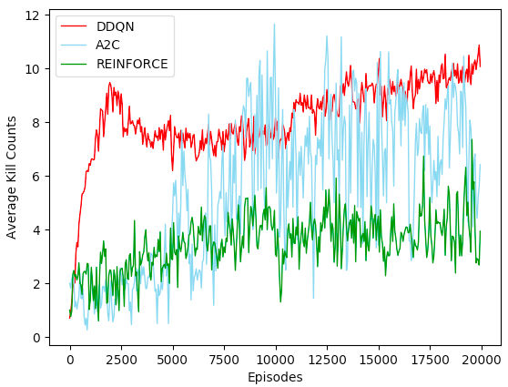
At first glance, I was surprised by the fact that DDQN worked so well as compared to Policy Gradients methods. DDQN was able to converge to a pretty good policy in the first 1000 episode, while A2C and REINFORCE took almost 5000 epsides to converge. This concurs with the theory that DDQN has higher data efficiency than Poliy Gradients. We simply need a lot of data to get Policy Gradients to work. Hence if we have restriction on the amount of data we can collect, we should probably not choose Policy Gradients. Another interesting thing to note, though not quite surprising, is that DDQN showed a very stable performance improved steadily over time, while A2C’s performance fluctuated from episode to episode. However, despite its variance, A2C was able to reach a higher maximum average kills (around 12) than DDQN (around 11).

Furthermore, it’s interesting to point out that DDQN and A2C have independently discovered 2 different strategies to play the game.

DDQN agent playing an episode

A2C agent playing an episode

We observe that A2C agent learned to only turn in one direction (i.e. Left) and refrained itself from shooting far away targets. This is contrasted by DDQN agent which wiggled a lot and tried to shoot whenever an enemy is within its sight, regardless of its distance. I think the strategy adopted by the Policy Gradients agent makes more sense and is more similar to the way human would approach the game. It’d better to shoot from close range to avoid missing the target and waste ammo.

Conclusions

This implementation exercise allows me to have a firmer grasp and more intuitive understanding of Q Learning and Policy Gradients. If time allows, I would love to port my implementation to even more challenging environment such as VizDoom Death Match scenario. In this scenario, the agent has to learn to shoot enemies while navigate in a challenging 3D maze at the same time. In fact, I have briefly tested out A2C on the Death Match scenario but failed to get any fruitful results. The state space and complexity of the environment might be too big for naive implementation to work. A rule of thumb, as pointed out by John Schulman in this lecture slides, is that if a random agent cannot achieve its goal on occasion, naive reinforcement learning will most likely not work. Some kind of curriculum learning or supervised pre-training by human demonstration might be necessary to get reinforcement learning to work in such environment.

P.S. In addition to DDQN, A2C and REINFORCE, I also implemented Dueling DDQN, Deep Recurrent Q Network (DRQN) with LSTM, A2C with LSTM, and C51 DDQN (Distributional Bellman). They all showed varying level of improvements over the original versions. I decided not to include them in the analysis. Interested readers can find all the implementations in this github.

I’ve also written a seperate blog post on analyzing C51 Distributional Bellman. Feel free to check it out!

Acknowledgement

I want to thank the Vizdoom Team for providing such a great environment and being so responsive to my emails. I also want to thank @yanpanlau for introducing me to VizDoom and provided useful feedbacks.

If you have any questions or thoughts feel free to leave a comment below.

You can also follow me on Twitter at @flyyufelix.