I recently took part in the Nature Conservancy Fisheries Monitoring Competition organized by Kaggle. Of all the image related competitions I took part before, this is by far the toughest but most interesting competition in many regards. I managed to finish in the 3rd place in public leaderboard but dropped to 8th place in the private leaderboard. I will go over my solution and lessons learned in detail and hopefully they will be useful to someone who come across with similar problems.

Problem Statement

The competition is organized by the Nature Observatory, with the meaningful objective of finding better ways to monitor unregulated fishing activities that are threatening marine ecosystems and global seafood supplies. Given a dataset of camera images taken from fishing boats, our goal is to develop algorithms to automatically detect and classify species of fish that the boats catch. This will lead to faster and more reliable video review which enables countries to better allocate human capital to management and enforcement activities.

Dataset

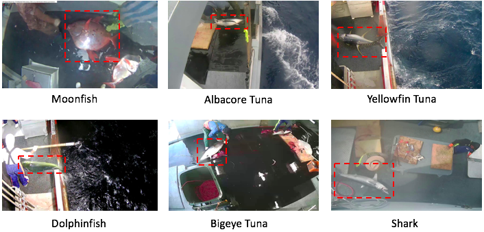
We are given a training dataset of 3792 images and testing dataset of 1000 images taken from fixed cameras mounted on fish boats. Our goal is to develop models to detect and classify the species of fish into the following 8 classes.

• Albacore Tuna
• Bigeye Tuna
• Dolphinfish
• Moonfish
• Shark
• Yellowfin Tuna
• Others
• No Fish

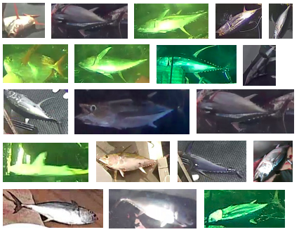
Here are the samples of images given to us (with location of the fish marked by a red box) :

The competition consists of 2 stages. In the first stage, we were provided with 1000 testing images. A public leaderboard score was computed based on results on that 1000 testing images. By the end of the first stage, we have to submit our models to Kaggle. The submitted models were frozen so we could not make any changes anymore. The second stage then began where a private testing dataset was released for us to ran our models on. The private ranking will be based entirely on the private testing data.

The evaluation metric is multi-class cross entropy loss (also called logarithmic loss)

Exploration

After running some simple exploration scripts, I quickly found out that there are a few aspects of this dataset which makes the competition extremely challenging.

1) Class Distribution is Highly Unbalanced

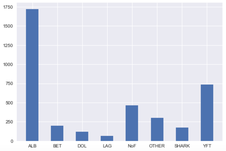
From the class distribution histogram above, we can see that “ALB” class has 1719 samples, which is roughly 45% of the training data, whereas “LAG” and “DOL” classes have only 67 and 117 samples respectively. As a result, the model might have trouble classifying those classes with very few training samples. We have to be very careful when splitting the training set into different folds for cross validation so that the model is able to “see” enough of the rare classes for each fold (i.e. Stratified K-fold).

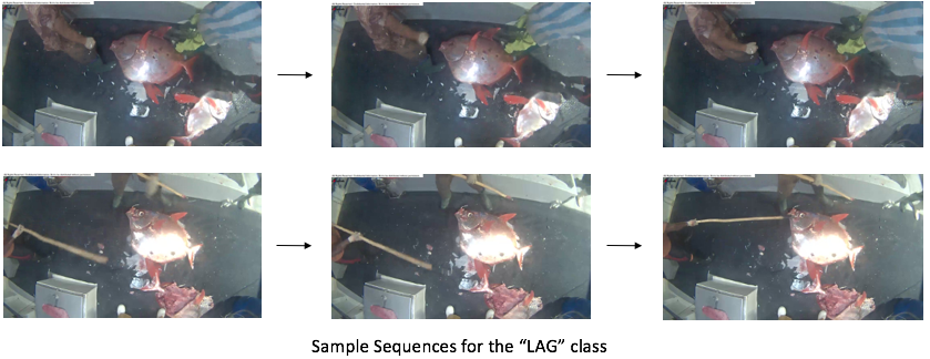
2) Samples Lack Diversity

I ran a simple clustering algorithm on downsampled (60x80) images and found out that there exists many highly correlated images within the same cluster. This is not surprising since many images are taken directly from video frame sequences. To put things into perspective, If we were to cut out the similar images, “LAG” class only has slightly more than 30 images. The same problem happens to a few other rare classes such as “DOL”, “SHARK” and “OTHER”.

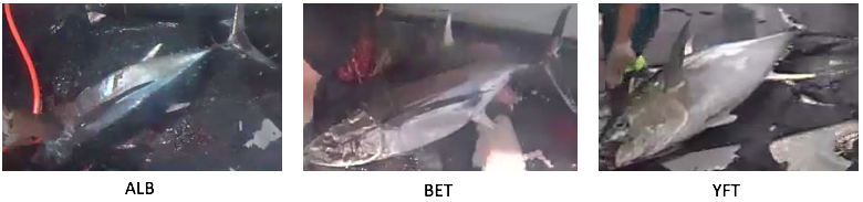
3) Ambiguous Classes

Some classes, say, “ALB”, “BET” and “YFT”, are extremely similar to each other. Even human cannot tell the difference between the those classes for many of the samples. Can you tell the difference between the 3 images which belongs to 3 different classes below? Lack of training data can only further aggravates the problem.

4) Noisy Labels

Upon some eyeball inspection, I discovered that many training samples were mislabeled. Since the evaluation metric is logarithmic loss, a confident but wrong answer will suffer a huge penalty (i.e. -log(0) -> infinity). Some contestants suggested manual relabeling of the training data and train the model on the relabeled data. However, in my opinion, this is a very dangerous practice since we don’t know if the test set contains any wrong labels or not. What if it does, then our model that trained on re-labeled data will give an even more confident prediction on the mislabeled images. This would drag down the score significantly. There was nothing much we can do to circumvent this problem but to accept the fact that things aren’t perfect (just like in real life!). However, we could minimize the impact of mislabeled data through clipping the prediction to a certain range (say 0.02 - 0.98) so that confident but wrong answers do not get penalized so much.

First Attempt: Pretrained ConvNets on Full Image

My first attempt was to naively throw the images into pretrained ConvNets and continue running gradient descent on our dataset, a process known as finetuning. This competition allows the use of pretrained models so throughout the competition I have made heavy use of pretrained models both for object detection and classification. I finetuned several different ConvNet models, including VGG-16/19, ResNet-50/152, Inception-V1 (GoogLeNet), Inception-V3/V4, Xception, DenseNet-121, ResNeXt-50/152. Stochastic Gradient Descent was used as the optimizer. The finetune procedure I used was similar to the one being used in the StateFarm Challenge. It’s very convenient to set up finetuning pipeline in Keras. I have open sourced our templating codes that perform finetuning on well known ConvNet models. It is implemented in Keras and that all models come with pretrained weights trained on ImageNet. For those who are interested to know more about finetuning, you can check out this post. Data augmentation strategies like rotation, translation, scaling, channel shifts, and flipping were performed.

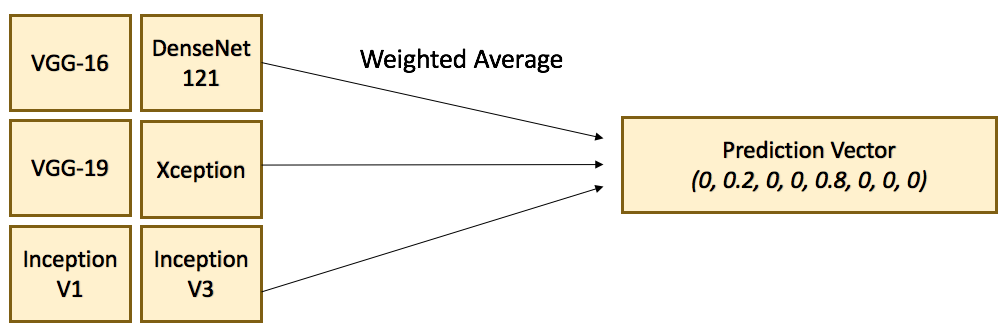
Out of my surprise, VGG-16 was our best performing single model for classification on full images. With 5 fold stratified CV, the model achieved a leaderboard logloss score of 0.84. ResNet models have the best local validation score but failed miserably on the public test set. I trained a few VGG models with varying input dimensions and ensemble them with other models with weighted averaging. The ensembled model achieved a logloss score of 0.73, which was pretty decent considering the fact that we have not explored localization yet. Below is the Ensemble Diagram.

I speculated that the good score was due to correlation between boat and fish types. Essentially, the model memorized some boat features in addition to the fish features. To test such hypothesis, I trained a variation of VGG-16 called VGG-CAM that allowed us to visualize which part of the image the model “look at” to make prediction decisions. VGG-CAM works by replacing the fully connected layers of VGG by global averaging layers called Class Activation Maps (CAM). Each map corresponds to a particular fish class. Through projecting the activation patterns of activation maps back to the input image, we could obtain heatmap like intensity which told us which part of the image the model focused on.

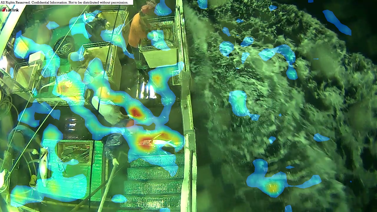
From the image above, We can see that the model put a lot of emphasis on features other than fishes. This is bad since this implies the model would fail miserably on unseen boats. In order to train a robust model that can generalize well on unseen boats we have to develop ways to localize the fish from the boat background before performing classification.

Detection and Localization

At this point, it became clear that in order to go further in the competition, we have to develop automated ways to crop out the fish from the images and perform classification on the crops. Someone has generously provided bounding box annotations on the entire training set in Kaggle forum (Thanks!) using a convenient tool called Sloth. We were all set to train our own detection model.

Bounding Box Regression

My first attempt was a simple bounding box regressor using pretrained VGG-16. I used a multi-part loss function which combines logloss (classification error) and mean squared error (bounding box regression error). The model failed to converge in the beginning. Only after I used a smaller learning rate did the model converge, but at a very slow rate after the first few iterations. I also tried using normalized bounding box coordinates for training but it didn’t make any difference, so I decided to stick with raw coordinate values.

I trained the model with 5-fold cross validation with data augmentation (rotation, flipping etc) and test time augmentation. To test the quality of the model, I plotted the predicted bounding box on the validation set as a histogram of Intersection Over Union (IOU).

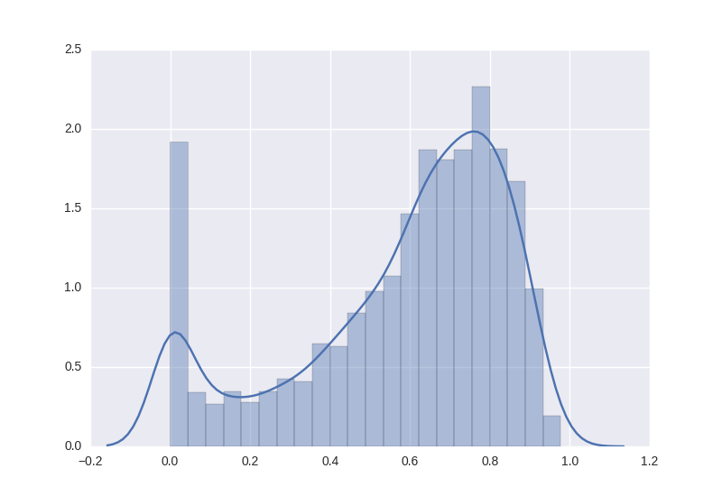
As seen from the histogram, the model was able to make somewhat intelligent predictions most of the time, despite complete failure with a small group of images (see the long bar at zero IOU). I then trained a ResNet-50 model on the cropped training images and ran it on the crops generated by our detector model. It achieved a logloss of 1.13, which was a lot worse than that of the full boat image. This was somewhat surprising to me since I thought the score would improve without being affected by the noise from the boat background. I thought the bad score was caused by the failure of the detector to correctly localize fishes for some (actually many) images, and those confident but wrong predictions got severly punished in logloss. Moreover, I found out that bounding box regression broke down completely on unseen boats. This was not surprising since such model generated the predicted coordinates based on features extracted from the entire input image, with no regional information incorporated. Hence the model tended to just memorize the boat in the background rather than recognizing the fish.

State-of-the-art Object Detection Models

It turns out that some very smart people from academia and industry have been working on object detection for years, and have developed some fascinated object detection models that works extremely well. I have previously heard of those models but never get the chance to try them out. This is a great opportunity to get my hands dirty and to apply them to our problem. There are plenty of object detection models out there, each have its own pros and cons. I have picked 3 models to try out. Below is a brief summary of the 3 models and my experience using them.

1) Faster R-CNN

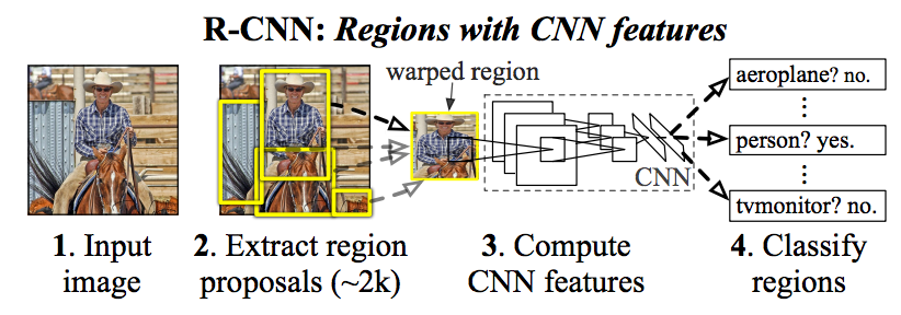
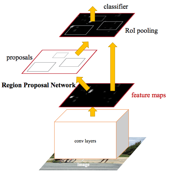
Faster R-CNN is an improved version of R-CNN (Region-based Convolutional Neural Networks). The basic idea is to break down object detection into a 2 separate stages. In the first stage, regions within the image that are likely to contain our object of interest are identified. In the second stage, a convolutional neural network is run on each proposed region and outputs the object category score and the corresponding bounding box coordinates that contains the object. The original version of R-CNN uses selective search to generate proposed regions for the first stage, then uses a pretrained VGG-16 to extract features from the proposed region and feeds those features into SVM to generate the final predictions.

Faster R-CNN is a drastically improved version of R-CNN that is way faster and more accurate. One of the major modifications of Faster R-CNN is to use Convolutional Neural Network to generate the object proposals as opposed to Selective Search in the first stage. It is called RPN (Region Proposal Network). On a high level, RPN first uses a base network (e.g. VGG-16, ResNet-101 etc) to extract features (more precisely, feature maps) from the image. It then partitions the feature maps into multiple squared tiles and slide a small network across each tile successively. The small network assigns a set of object confidence scores and bounding box coordinates to each tile location. Notice that the RPN designed to be trained end-to-end in a fully convolutional manner. Below is an illustration of RPN from a diagram.

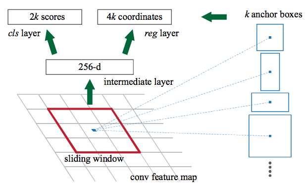
RPN by itself is already a very strong object detector. The second stage, which is commonly known as “pixel resampling”, fits another small network on top of each proposed region generated by RPN and output a set of refined category scores and bounding box coordinates for that region. It basically serves as a “refinement” to the results of RPN.

Faster R-CNN is the current state-of-the-art model with the best mAP scores on the VOC and COCO benchmarks. However, with a framerate of 7 fps, Faster R-CNN is the slowest amongst other state-of-the-art models such as YOLO and SSD, which I will cover in later part of this blog post. This is also the major drawback of Faster R-CNN.

Another notable architecture that also resembles Faster R-CNN’s 2 stage process is F-RCN. Both models use RPN for the first stage. They differ in the second stage where F-RCN applies ROI pooling to the last layer, as opposed to Faster R-CNN which applies ROI pooling from the same layer where region proposals are predicted. As a result, F-RCN can be trained and makes inference in a single pass convolutional manner, and thus runs significantly faster than Faster R-CNN while having comparable accuracy. However, since running time is not a major concern for this competition I decided to just stick with Faster R-CNN.

I trained a few variants of Faster R-CNN using this TensorFlow implementation on our fish data, one group uses VGG-16 as base networks, the other uses ResNet-101 as base networks. While several literature suggests that using ResNet-101 as feature extractors can increase accuracy, however, I did not notice any significant difference. For each image, I picked the object with the highest confidence score, cropped it out and saved it to a folder. Initially, I tasked the model with outputting multi-class object confidence scores (i.e. 7 classes excluding background class). But since the main purpose of the model is to locate and crop out the fish from the background, I figured the model might produce better crops by just assigning a binary fish or no fish label for training. Indeed, the quality of crops improved with binary labels. Below are samples of the crops generated by Faster R-CNN with ResNet-101 as feature extractor.

In fact, it is able localize the fish almost perfectly for most images, and is very robust on unseen boats.

2) YOLO (You Only Look Once)

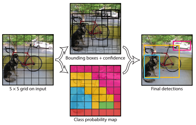
YOLO is another well known object detection model that is known for its simplicity and fast performance. As compared to 5 to 7 fps by Faster R-CNN, YOLO achieves a framerate of 45 fps. Hence, it is particularly well suited to real-time object detection tasks, such as object detection on streaming video. On a high level, YOLO first partitions the raw input image into NxN squared regions. Then it fits a convolutional neural network directly on the input image and output M sets of object confidence scores and bounding box coordinates, with M depending on N. The entire model is trained end-to-end.

Since YOLO takes raw image as input and output confidence scores and bounding box coordinates directly with a single pass, it is considerably faster than Faster R-CNN which requires multiple stages for training and inference. However, it’s fast speed comes as a price. It is significantly less accurate than Faster R-CNN, and is particularly bad at localizing small objects.

I used an improved version of YOLO called YOLO v2. It made several small but important changes inspired by Faster R-CNN, such as assigning bounding box coordinate “priors” to each partitioned region and replacing the fully connected layers with convolutional layers, hence making the network fully convolutional. Essentially, YOLO v2 works very similarly to RPN.

I used the original darknet implementation written (in C!!) by the creator of YOLO. Binary labels were used for training. For each image, I picked the object with the highest confidence score and saved it to a folder. Through manual eyeballing, the model was able to generate equally good crops on the public test set as Faster R-CNN.

3) SSD (Single Shot Multibox Detector)

SSD is another state-of-the-art object detection model that is known to have good tradeoff in speed and accuracy. Similar to YOLO, it requires only a single step for training and inference and the entire model is trained end-to-end. The major contribution of SSD as compared to other models is that it makes use of feature maps of different scales to generate predictions. In contract, Faster R-CNN and YOLO based their predictions only on a single set of feature maps located at some selected intermediate level (e.g. “conv5”) down the convolutional layers hierarchy. Theoretically speaking, using feature maps of varying scales can lead to better detection quality of objects with different sizes. Below is a diagram that illustrates the architecture of SSD and it’s different with that of YOLO.

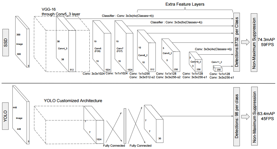
I trained a few SSD models using this Keras implementation. By default, it uses VGG-16 as feature extractor and takes 300x300 images as inputs. The model converged nicely. Again, for each image, we picked the object with the highest confidence score and saved it to a folder. For curiosity sake, I also implemented my own ResNet-101 with Feature Pyramidal Network (FPN) in Keras and used it to replace the VGG-16 base network. However, much to my dismay, the new architecture did not yield any improvement.

Performance Comparison

I trained a ResNet-50 model on the training crops and ran it on the testing crops generated by our detector models. All 3 models, Faster R-CNN, YOLO, and SSD, outperformed our homebrew bounding box regressor by a huge margin. As discussed above, the bounding box regression model has a logloss of 1.13 on the public test set. In comparison, variants of Faster R-CNN and YOLO achieved logloss that ranges from 0.5x to 0.6x, while SSD has slightly worse scores that ranges from 0.7x to 0.8x. I also carried out manual eyeballing of the quality of the cropped images. Faster R-CNN and YOLO have the best quality crops, while SSD predictions are noticeably inferior, especially on the harder samples.

I personally think that input resolution plays an important role in localization accuracy. Essentially, I only used 300x300 inputs for the SSD implementation. On the other hand YOLO accepts 448x448 inputs and Faster R-CNN rescales inputs to 600 pixels on the shorter side.

This paper conducts a comprehensive study on the comparison of performance for Faster R-CNN, F-RCN, and SSD. Indeed, input resolution does play an important part in localization accuracy, especially on small objects.

Robustness

Towards later part of the competition I tested the object detectors on a selected validation set of unseen boats. This is to gauge whether the detectors can generalize well to unseen data. Much to my surprise, I found out that while Faster R-CNN was able to correctly locate most of the fishes, YOLO and SSD broke down quite badly.

I think this is very much related to how the respective models works. As discussed above, Faster R-CNN uses a 2 staged process in training and inference. The first stage makes use of RPN to generate object proposals. The second stage (pixel resampling step) serves as a refinement to RPN. In contrast, YOLO and SSD generates predictions directly from raw inputs just like the RPN, but lacks the refinement step which uses information on local regions. Without the refinement step, YOLO and SSD’s predictions relies more heavily on background information, which leads to its breaking down on new boat background.

After discovering this, I decided to abandon all SSD models, downwardly adjusted the weighting of YOLO and placed most emphasis on Faster R-CNN.

Classification Models

So now we are in possession of a pretty good object detector that can locate and crop out the fishes with reasonable robustness. Our next step is to train a good classifier that can accurately identify the fish species. In addition to ResNet-50, I tested out different architectures such as ResNet-101/152, DenseNet-121/161, ResNeXt-101/152, Xception, and VGG-16/19 on the validation set, and picked the models with the best validation and leaderboard scores for ensembling.

Port Caffe Models to Keras

Since I wrote the classification pipeline in Keras, I would love to have the above models implemented in Keras as well. Unfortunately, most of the pretrained models only available in Caffe (protocol buffer format…) but not in Keras (this is the one thing I dislike about Keras!). This time, I managed to muster up the courage to convert Caffe models to Keras. The process was not as easy and straightforward as I thought. You can read my other post for a detail coverage of how to go about converting Caffe to Keras for ResNet-152. For those of you who are interested, I hosted the converted Keras schema and pretrained model for ResNet-152 (both Theano and TensorFlow backend) here. I did the same thing for DenseNet and ResNeXt too but didn’t have the time to organize the schema and post the code yet.

I trained the models with stratified 5 Fold CV with data augmentation for both training and test time. ResNet-152 and DenseNet-121 have the best overall performance on the validation and public test set, so I ended up choosing them for the final ensemble model. In retrospect, I did not put together a validation set on new boats until very late in the competition (more on it in the “Lesson” section below). I discovered that ResNet-152 has a tendency to spit out very confident predictions. If the private test set consists of primiarily new boats, ResNet-152 might give confident but wrong answers, which is exactly what we want to avoid for logloss metric. I think my private score would have improved significantly if I validated the models on new boats.

Use of External Data

External data is allowed for this competition. Like many other contestants, I handpicked around 100 images from ImageNet, mostly for the rare classes (i.e. DOL, LAG, OTHER, and SHARK) and used them to train the objection detection and classification models. The use of external data did improve the score a little bit, but not by much.

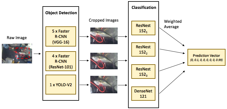
Our Final Ensembled Model

The final ensemble consists of the following classification models:

• 3 x ResNet-152 (different input resolutions and data augmentation strategies)
• 1 x DenseNet-121

For each of the above model, generates 1 set of prediction on each set of crops generated by the following object detection models:

• 1 x YOLO
• 3 x Faster R-CNN with ResNet-101 as base network (different training iterations)
• 4 x Faster R-CNN with VGG-16 as base network (different training iterations)
• 1 x Faster R-CNN with VGG-16 as base network (trained with multi-class labels)

We then merged together all the prediction files by weighted averaging.

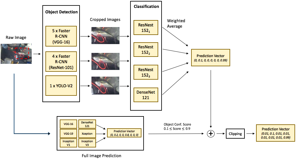
Incorporate Boat Information as “Prior”

As discussed above, since the boat background is correlated with the fish type, it might be advantageous to incorporate boat information to the model. I reasoned that in the cases where the object detectors fail to locate the fish (i.e. crop out garbage), the boat information could act as a “prior” to smooth out the probabilities. Hence I used the following trick. For a particular image, If the object detector was not so confident about its prediction (i.e. return a low objectness score), I merged the crop prediction with the full image prediction by weighted averaging. In fact, this trick works very well both on our validation set and public test set. However, this trick proved to be disastrous for the 2nd stage private test data which consists of unseen and very different boats. This is one of the costliest gamble I made but unfortunately it went the wrong direction.

Post Processing

I decided to clip predictions to a lower bound of 0.01. This was to avoid heavy penalty of confident but wrong answers given by the logloss metric (i.e. -log(0) -> infinity). In addition, I used a higher clipping constant of 0.05 for the “BET” and “YFT” classes for cases where the prediction of “ALB” is high (i.e. > 0.9), since “ALB”, “BET”, and “YFT” classes are very similar with many samples highly indistinguishable from one another.

With boat information and clipping, the full model diagram looks like this.

Other Methods

There were several other methods I have tried but didn’t work well enough to be used in the final solution. It’s worthwhile to briefly go over them here.

1) Feature Pyramidal Network (FPN)

FPN is a novel architecture that was recently introduced by Facebook for object detection. It is specifically designed to detect objects at different scales by using skip connections to combine l model diagram looks like tales. The idea is very similar to that of SSD. Using FPN with ResNet-101 as the base network for Faster R-CNN achieves the current state-of-the-art single model results on the COCO benchmark. In addition, the model has a framerate of 5 fps, which is good enough for use in most practical applications.

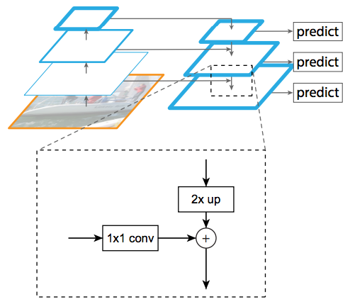
I created my own implementation of FPN with ResNet-101 in Keras and plugged it into SSD. Since FPN uses skip connections to combine feature maps at different scales, it should generate better quality predictions than that of SSD which doesn’t leverage skip connections. I anticipated that FPN would be better at detecting fishes at extreme scales (either extremely big or small). However, though the model somehow managed to converge, it didn’t work as well as expected. I would have to leave it for further investigation.

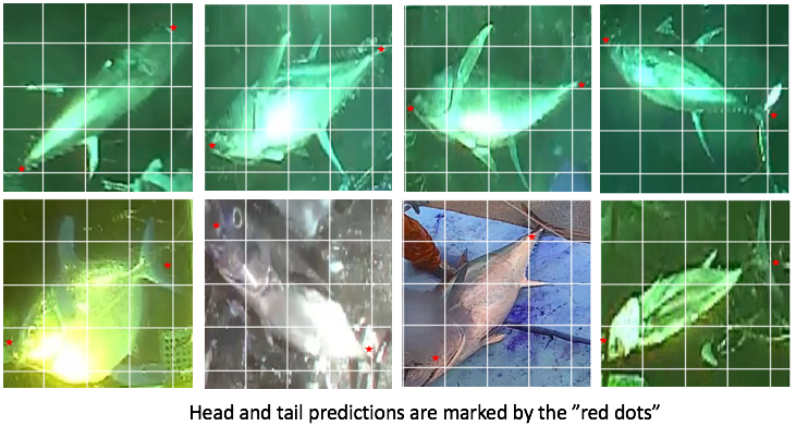
2) Head Tail Rotational Alignment

There was another similar Kaggle competition on classifying whale species where the winners adopted a novel trick to rotate and align the body of the whale so that their head always point to the same direction, creating a “passport” photo. This trick worked extremely well for that competition. That makes sense since convolutional neural network is rotational variant (well, pooling might alleviate the problem a little bit), aligning the object of interest to the same orientation should improve classification accuracy.

I decided to apply the same trick for our problem. Someone has annotated the head and tail position for each image and posted the annotation in the forum (thanks!). Initially, I used the annotation to train a VGG-16 regressor that directly predicts head and tail positions from the full image. Needless to say it failed miserably. I then trained another VGG-16 regressor to predicts head and tail positions from cropped images, and it worked extremely well. Our regressor can predicts the exact head and tail positions almost perfectly, as indicated by the “red dots” from the images below!

I then rotated the cropped images so that their head and tail horizontally aligned. Below are samples of rotated samples.

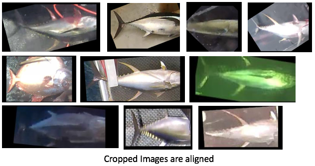
Surprisingly, classifying on the rotationally aligned images did not improve our results at all. I think this is because of the fact that all images are taken from a fixed camera angle on the boats. Hence, the fishes are placed in similar positions and are orientated similarly. Rotationally alignment would not add much new information.

Lessons

1) The importance of establishing a GOOD Local Validation!!!

Having competed in multiple competitions, this is, in my opinion, the most important factor for achieving top results on a consistent basis in Kaggle. Before jumping right into the model, it’s worthwhile to put some serious thoughts on how to go about establishing a representable and stable validation scheme. We certainly learned it the hard way multiple times. Fair to say I did get lucky once, made a significantly jump to get into top 10 in the private leaderboard for that one time. But unfortunately for a 2 stage competition like this one and with a lack of information on the private set, it’s extremely tough to establish a good and stable local benchmark.

Throughout most of the competition, I used a stratified 5 fold cross validation for validating results locally. I did not use unseen boat for validation (until the last 2 weeks) for the following 2 reasons.

First, since classes are distributed very unevenly (“LAG” class only has 76 samples, “DOL”, “SHARK” and “OTHER” all have very few training samples), if we partition the training data into different set of boats (also distributed very unevenly) for validation, the model might miss out completely on those rare class training samples, and that the validation result would be very bad and unrepresentative.

Second, the organizers did not tell us whether the 2nd stage private data would contain new boats or not and what’s the ratio of new boats vs existing boats. Since the samples from public test set are all from existing boats I naively thought that the majority of the images from the private test set, if not all, would be from existing boats too. Not until 2 weeks from the end of the competition did the organizer tell us that the private test set would contain new boats (still we don’t know the ratio of new vs old).

So after I was informed that the private test set will have new boats, I hastily put together a new validation set with unseen boats to minimize the impact of potential overfitting. First I used the new validation set on object detection models, and ended up abandoning all of the SSD models and most of the YOLO models. Next, I used the new validation set on the classification models. The validation results was pretty bad. However, there were only a few days remaining for the competition, there simply wasn’t enough time for me to test out and retrain all the models. Also, I still somehow thought that significantly portion of the private test set would be from existing boats. I was so wrong! It turned out that all 12000+ images from the private test set are from unseen and very different boats!

To put things into perspective, a simple change to a constant so that less emphasis is placed on the boat information “priors” would get me to jump 3 positions on the private leaderboard to the 5th place!

2) Limitation of Deep Learning with very few labeled data

The private dataset consists of 12000+ images on unseen and very different boats. The quality and scale of the fishes also differ significantly from those in the training set. As a result, the logloss scores in the private leaderboard was a lot worse than that of the public leaderboard. I think this is a good case that exposes the weaknesses of Deep Learning.

With very few training data, ConvNet is quite incapable of recognizing and making decisions based on subtle features from the fishes. For example, “ALB” and “YFT” can be told apart by the length and curve of the dorsal and anal fins. Human can easily tell the difference by just seeing a couple of sample images, even if part of the fins are not visible, or got blocked by obstacles. However, the ConvNet models failed quite badly whenever part of the fins got slightly blocked or being obscured by say a spray of water. Deep Learning models do not possess the kind of “common sense” that human possesses. They are incapable of making logical deduction based on the ontology of the physical world. This remains an active and important area of research for general artificial intelligence.

Acknowledgement

I want to thank Kaggle and the Nature Conservancy for organizing this interesting and challenging competition. This was a great and unique learning opportunity for me. I also want to thank fellow participants who shared insightful comments and their approaches on forum. Those discussions certainly helped me a lot. And of course those who spent the time to annotate the fishes manually and kindly release the annotations for our use. Your efforts are greatly appreciated.

If you have any questions or thoughts feel free to leave a comment below.

You can also follow me on Twitter at @flyyufelix.