I got the chance to read this paper on Distributional Bellman published by DeepMind in July. Glossing over it the first time, my impression was that it would be an important paper, since the theory was sound and the experimental results were promising. However, it did not generate as much noise in the reinforcement learning community as I would have hoped. Nevertheless, as I thought the idea of Distributional Bellman was pretty neat, I decided to implement it (in Keras) and test it out myself. I hope this article can help interested readers better understanding the core concepts of Distributional Bellman.
Q Learning Recap
To understand Distributional Bellman, we first have to acquire a basic understanding of Q Learning. For those of you are are not familiar with Q Learning, you can refer to my previous blog for more information on the subject. To recap, the objective of Q Learning is to approximate the Q function, which is the expected value of the total future rewards by following policy \(\pi\).
\[Q^{\pi}(s,a) = E[R_t]\]where \(\pi\) refers to the policy, \(s\) represents the state input and \(a\) is an action chosen by the policy \(\pi\) at state \(s\). \(R_t\) is the sum of discounted future rewards.
\[R_t = r_t + \gamma r_{t+1} + \gamma^2 r_{t+2} + ...\]At the center of Q Learning is what is known as Bellman equation. Let \(\pi^*\) represents the optimal policy. We sample a transition from the environment and obtain <\(s\), \(a\), \(r\), \(s^\prime\)>, where \(s^\prime\) is the next state. The Bellman equation is a recursive expression that relates the Q functions of consecutive time steps.
\[Q^{\pi^*}(s,a) = r + \gamma\max_{a^\prime} Q(s^\prime,a^\prime)\]Why is it so important? Bellman equation basically allows us to iteratively approximate the Q function through temporal difference learning. Specially, at each iteration, we seek to minimize the the mean squared error of the \(Q(s,a)\) (prediction term) and \(r + \gamma\max_{a^\prime} Q(s^\prime,a^\prime)\) (target term)
\[L = \frac{1}{2}[r + \gamma\max_{a^\prime} Q(s^\prime,a^\prime) - Q(s,a)]\]In practice, we usually use a deep neural network as the Q function approximator and applies gradient descent to minimize the objective function \(L\). This is known as Deep Q Learning (DQN). Once we obtain a reasonably accurate Q function, we can obtain the optimal policy through
\[\pi^*(s) = arg\!\max_a Q(s,a)\]That’s all we need to know about Q Learning. Let’s get to Distributional Bellman now.
So What Exactly is Distributional Bellman?
The core idea of Distributional Bellman is to ask the following questions. If we can model the Distribution of the total future rewards, why restrict ourselves to the expected value (i.e. Q function)? There are several benefits to learning an approximate distribution rather than its approximate expectation.
Consider a commuter who drives to work every morning. We want to model the total commute time of the trip. Under normal circumstances, the traffic are cleared and the trip would take around 30 minutes. However, traffic accidents do occur once in a while (e.g. car crashes, break down in the middle of the highway, etc), and if that happens, it will usually cause the traffic to be at a standstill and add an hour to the trip (i.e. 90 minutes). Let’s say traffic accident like that happens once every 5 days on average. If we use expected value to model the commute time of the trip, the expected commute time will be 30 + 60 / 5 = 42 minutes. However, we know such expected figure is not so meaningful, since it vastly overestimates the commute time most of the time, and vastly underestimates the commute time when traffic accidents do occur. If instead we treat the total commute time as a random variable and model its distribution, it should look like this:
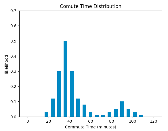
Notice that the distribution of commute time is bimodal. Most of the time the trip would take 30 minutes on average, however, if traffic accident occurs, the commute time would take 90 minutes on average. Given the full picture of the distribution, next time when we head out to work, we’d better look up the traffic situation on the highway. If traffic accident is reported, we can choose to bike to work which would take around 60 minutes, which could save us 30 minutes!
Choosing Action based on Distribution instead of Expected Value
In reinforcement learning, we use the Bellman equation to approximate the expected value of future rewards. As illustrated in the commute time example above, if the environment is stochastic in nature (occurrence of traffic accidents) and the future rewards follow multimodal distribution (bimodally distributed commute time), choosing actions based on expected value may lead to suboptimal outcome. In the example above, if we realize there is a traffic accident and it will likely take 90 minutes to get to office, the optimal action would be to bike even though the expected commute time of biking is 60 minutes which is larger than the expected commute time of driving (42 minutes).
Another obvious benefit of modeling distribution instead of expected value is that sometimes even though the expected future rewards of 2 actions are identical, their variances might be very different. If we are risk averse, it would be preferable to choose the action with smaller variance. Using the commute time example again, if we have 2 actions to choose from: driving or taking the train, both actions have the same expected commute time (i.e. 42 minutes), but taking the train has smaller variance since it does not get affected by unexpected traffic conditions. Most people would prefer taking the train over driving.
Formulation of Distribution Bellman
Without further due, let’s get to the definition of Distributional Bellman. It’s actually quite simple and elegant. We simply use a random variable \(Z(s,a)\) to replace \(Q(s,a)\) in the Bellman equation. Notice that \(Z\) represents the distribution of future rewards, which is no longer a scalar quanity like Q. Then we obtain the distributional version of Bellman equation as follows:
\[Z(s,a) = r + \gamma Z(s^\prime,a^\prime)\]This is called the Distributional Bellman equation, and the random variable \(Z\) is called the Value Distribution. A caveat is that the equal sign here means the 2 distributions are equivalent. In the paper the author applied Wasserstein Metric to describe the distance between 2 probability distributions and proved the convergence of the above distributional Bellman equation. I am not going to go through the mathematical details. Interested readers can find the proof in the paper.
Similar to Q Learning, we can now use the Distributional Bellman equation to iteratively approximate the value distribution \(Z\). Sounds easy enough. But before we do that, there are 2 issues we have to address. The first issue is how to represent the value distribution \(Z\) since it’s not a scalar quantity like Q? The second issue is how to “minimize the distance” between the 2 value distributions \(Z\) and \(Z^\prime\) so that temporal difference learning can be performed?
To address our first concern, the paper proposed the use of a discrete distribution parameterized by the number of supports (i.e. discrete values) to represent the value distribution \(Z\). For example, if the number of supports equals 10, then the domain of the distribution will be 10 discrete values uniformly spaced over an interval. This discrete distribution has the advantages of being highly expressive (i.e. it can represents any kind of distributions, not limited to Gaussian) and computationally friendly. Moreover, Cross Entropy loss can be used to quantify the distance between 2 discrete distributions \(Z\) and \(Z^\prime\), since they share the same set of discrete supports.
Here is a visual representation of the update step of Distributional Bellman equation:
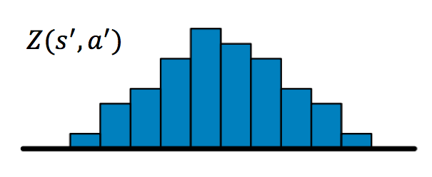
First we sample a transition from state \(s\) with action \(a\) and obtain next state \(s^\prime\) and reward \(r\). The next state distribution \(Z(s^\prime,a^\prime)\) looks like this
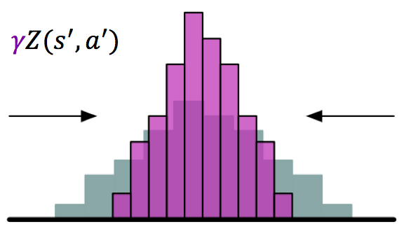
We then scale the next state distribution with \(\gamma\) and shift the resulting distribution to the right by \(r\) to obtain our target distribution \(Z^\prime = r + \gamma Z(s^\prime,a^\prime)\)
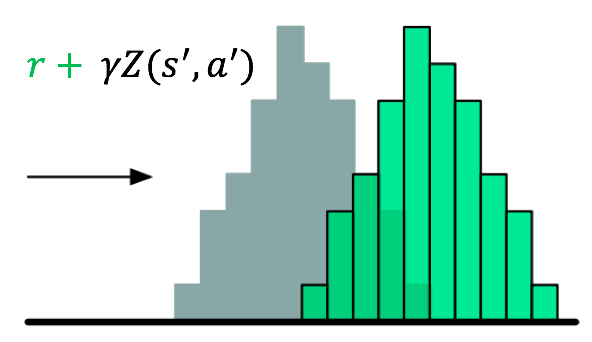
Last of all, we “project” the target distribution \(Z^\prime\) to the supports of the current distribution \(Z\) simply by minimizing the cross entropy loss between \(Z\) and \(Z^\prime\).
Intuitively, we can view this as an image classification problem. The inputs to the model can be screen pixels sampled from game play (e.g. Atari Pong, Breakout, etc). Each discrete support of \(Z\) represents a unique “category”. During the update step, the probability mass of each “category” of \(Z^\prime\) will serve as “fake ground truth labels” to guide the training. The “fake labels” are analogous to the binary ground truth labels we use for classification problems.
Now it’s time to go through the meat of this article, which is a feasible algorithm to implement Distributional Bellman called C51.
Categorical “C51” Algorithm
C51 is a feasible algorithm proposed in the paper to perform iterative approximation of the value distribution Z using Distributional Bellman equation. The number 51 represents the use of 51 discrete values to parameterize the value distribution \(Z\). Why 51 you may ask? This is because the author of the paper tried out different values and found 51 to have good empirical performance. We will just treat it as the magic number.
C51 works like this. During each update step, we sample a transition from the environment and compute the target distribution \(Z^\prime\) (i.e. scale the next state distribution by \(\gamma\) and shift it by reward \(r\)), and uses \(Z^\prime\) to update the current distribution \(Z\) by minimizing the cross entropy loss between \(Z\) and \(Z^\prime\). The pseudo code of C51 Algorithm is provided by the paper:
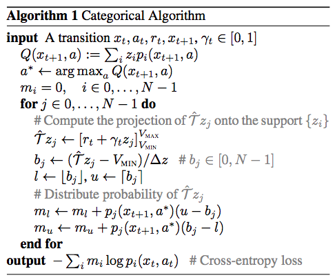
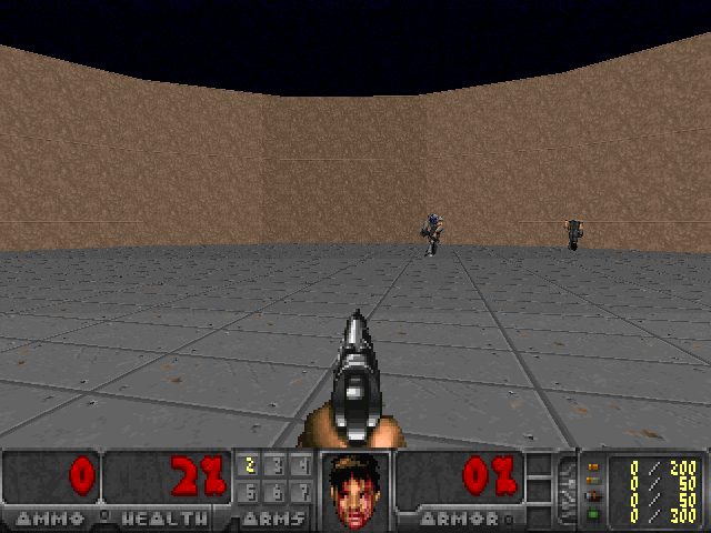
Look a bit confused? No worries. I have implemented C51 in Keras (code can be found here) which you can freely reference. The implementaion is tested on the VizDoom Defend the Center scenario, which is a 3D partially observation environment.
VizDoom Defend the Center Environment
In this environment, the agent occupies the center of a circular arena. Enemies continuously got spawned from far away and gradually move closer to the agent until they are close enough to attack from close range. The agent is equipped with a handgun. With limited bullets (26 in total) and health, its objective is to eliminate as many enemies as possible while avoid being attacked and killed. By default, a death penalty of -1 is provided by the environment. In order to facilitate learning, I enriched the variety of rewards (reward shaping) to include a +1 reward for every kill, and a -0.1 reward for losing ammo and health. I find such reward engineering trick to be quite crucial to get the agent to learn good policies.
C51 Keras Implementation
Let’s briefly walk through the implmentation. Similar to DQN, we first use a deep neural network to represent the value distribution \(Z\). Since the inputs are screen pixels, the first 3 layers are convolutional layers:
state_input = Input(shape=(input_shape))
cnn_feature = Convolution2D(32, 8, 8, subsample=(4,4), activation='relu')(state_input)
cnn_feature = Convolution2D(64, 4, 4, subsample=(2,2), activation='relu')(cnn_feature)
cnn_feature = Convolution2D(64, 3, 3, activation='relu')(cnn_feature)
cnn_feature = Flatten()(cnn_feature)
cnn_feature = Dense(512, activation='relu')(cnn_feature)
The neural network outputs 3 sets of value distribution predictions, one for each action (i.e. Turn Left, Turn Right, Shoot). Each set of prediction is a softmax layer with 51 units.
distribution_list = []
for i in range(action_size):
    distribution_list.append(Dense(num_atoms, activation='softmax')(cnn_feature))
For our problem the action_size is 3 (i.e. Turn Left, Turn Right, Shoot) and num_atoms is the number of discrete values (i.e. 51).
Most of the logic of the algorithm is contained in the update step. First we sample a minibatch of sample trajectories from the Experience Replay buffer and initialize the corresponding states, reward, and targets variables:
num_samples = min(self.batch_size * self.timestep_per_train, len(self.memory))
replay_samples = random.sample(self.memory, num_samples)

state_inputs = np.zeros(((num_samples,) + self.state_size))
next_states = np.zeros(((num_samples,) + self.state_size))
m_prob = [np.zeros((num_samples, self.num_atoms)) for i in range(action_size)]
action, reward, done = [], [], []

for i in range(num_samples):
    state_inputs[i,:,:,:] = replay_samples[i][0]
    action.append(replay_samples[i][1])
    reward.append(replay_samples[i][2])
    next_states[i,:,:,:] = replay_samples[i][3]
    done.append(replay_samples[i][4])
The variable m_prob stores the probability mass of the value distribution \(Z\).
Next, we carry out a forward pass to get the next state distributions.
z = self.model.predict(next_states)Notice that the model outputs 3 set of value distributions, one for each action. We really only need the one with the largest expected value to perform the update (similar to \(max_{a^\prime} Q(s^\prime,a^\prime)\) in Q Learning).
optimal_action_idxs = []
z_concat = np.vstack(z)
q = np.sum(np.multiply(z_concat, np.array(self.z)), axis=1) # length (num_atoms x num_actions)
q = q.reshape((num_samples, action_size), order='F')
optimal_action_idxs = np.argmax(q, axis=1)
We then compute target distribution \(Z^\prime\) (i.e. scale by \(\gamma\) and shift by reward \(r\)) and “project” it to the 51 discrete supports.
for i in range(num_samples):
    if done[i]: # Terminal State
        # Distribution collapses to a single point
        Tz = min(self.v_max, max(self.v_min, reward[i]))
        bj = (Tz - self.v_min) / self.delta_z
        m_l, m_u = math.floor(bj), math.ceil(bj)
        m_prob[action[i]][i][int(m_l)] += (m_u - bj)
        m_prob[action[i]][i][int(m_u)] += (bj - m_l)
    else:
        for j in range(self.num_atoms):
            Tz = min(self.v_max, max(self.v_min, reward[i] + self.gamma * self.z[j]))
            bj = (Tz - self.v_min) / self.delta_z
            m_l, m_u = math.floor(bj), math.ceil(bj)
            m_prob[action[i]][i][int(m_l)] += z_[optimal_action_idxs[i]][i][j] * (m_u - bj)
            m_prob[action[i]][i][int(m_u)] += z_[optimal_action_idxs[i]][i][j] * (bj - m_l)
Last, we call Keras fit() function to minimize the cross entropy loss with gradient descent.
loss = self.model.fit(state_inputs, m_prob, batch_size=self.batch_size, nb_epoch=1, verbose=0)That’s it! I strongly encourage you to try out the code in your favorite environment. Feel free to reach out to me if you have trouble getting to code to work.
Experiment
15,000 episodes of C51 was run on the VizDoom Defend the Center scenario. Average kill counts (moving average over 50 episodes) was used as the metric for performance. We really want to figure out 2 things. First, we want to know if C51 works on a non-trivial 3D partially observable environment. Second, we want to compare its performance with Double DQN (DDQN) and see if the result concurs with that of the paper.
Here is a video of C51 agent playing an episode
Here is the performance chart of C51 and DDQN
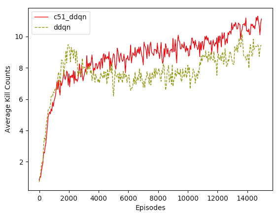
The first thing we notice is that C51 does work! A random agent can only get an average kill count of 1 by firing bullets randomly. In contrast, C51 was able to converge to a good policy pretty quickly and already reached an average kills of 7 in the first 1000 episodes. Even though learning started to slow down after episode 1000, we still see a steady and monotonic improvement over the remaining 14,000 episodes.
In addition to the performance chart, it is worthwhile to visually inspect the value distributions learned by C51 to gain a deeper understanding of how C51 works.
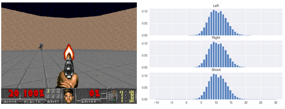
Figure 1: At the beginning of episode. Notice that the value distributions learned by C51 are very smooth and closely resemble Gaussian. Since there are still plenty of ammo left (bottom left corner indicates there are 20 left), individual actions (i.e. Turn Left, Turn Right, Shoot) should not affect the value distributions much. They pretty much look identical.
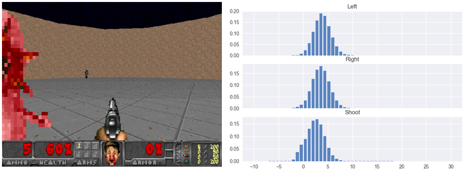
Figure 2: The episode progresses. A pink monster attacks from the left. Ammo starts to run out (5 left) so there is not much room to fire and miss the target. This is reflected by the “leftward shift” of the value distribution that belongs to shooting (bottom distribution). The decision to shoot and miss will certain result in 1 fewer kill.
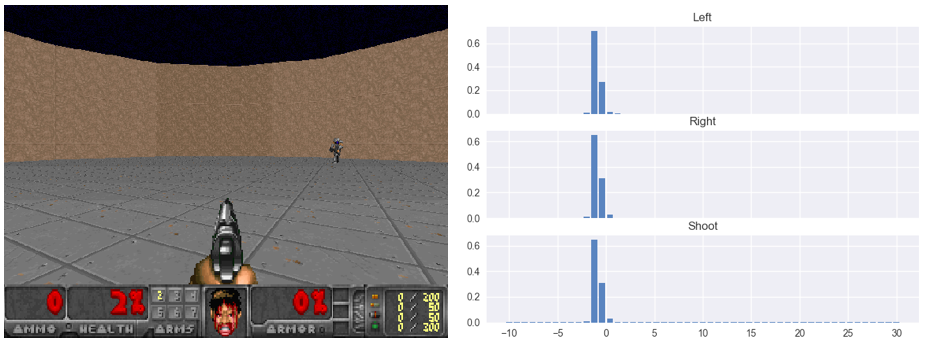
Figure 3: Towards the end of episode. Ammo runs out. Value distributions collpase to zero (actually slight negative since there is a negative reward at the end of the episode for getting killed)
It’s glad to see that the value distributions learned by C51 make sense and are highly interpretable. I strongly encourage you to plot out the distribution and check if they make sense for your particular environment, even if the algorithm works.
Comparison with DDQN
Now we answer our second question, which is how C51 stacks up against DDQN. We can see from the performance chart that C51 has a noticeable lead in average kills overall. Due to their similarly in nature (i.e. both rely on Bellman updates), their overall convergence rates and score variances are very similar. Both algorithms showed impressive convergence rate in the first 1000 episodes, DDQN even outperformed C51 briefly from episode 1000 to 3000. However, after episode 3000, C51 caught up and surpassed DDQN and have maintained that lead (around 1 to 2 average kills) for the remaining 1200 episodes. In fact, the gain in performance for C51 over DDQN is not as big as I would have expected, considering that the paper reported a doubling of performance on the Atari Learning Environment (ALE). Perhaps VizDoom Defend the Center is not the ideal environment to showcase the true power of Distributional Bellman.
Conclusion
In my opinion, Distributional Bellman is a very interesting and theoretically sound way to model reinforcement learning problem. As mentioned in the article and testified by many experiements, there are many benefits of modeling value distribution instead of the expected value. There is also a simple and feasible implementation C51 that consistently outperforms DDQN in both Atari and VizDoom environments. I would love to see higher adoption of distributional methods. Last of all, my Keras implementation of C51 can be found in my github. Feel free to use it for your own problem.
If you have any questions or thoughts feel free to leave a comment below.
You can also follow me on Twitter at @flyyufelix.