Instruct DFP agent to change objective (at test time) from pick up Health Packs (Left) to pick up Poision Jars (Right). The ability to pursue complex goals at test time is one of the major benefits of DFP.

In this post, I am going to go over a novel algorithm in reinforcement learning called Direct Future Prediction (DFP). In my opinion, it has a few really interesting properties that make it stand out from well known methods such as Actor Critic and Deep Q Learning. I will try my best to give my insights and walk you through my implementation on a scenario (VizDoom Health Gather) which I think is well suited to showcase DFP’s benefits.

Why should we care about DFP?

DFP first caught my attention when it won the ‘Full Deathmatch’ track of the VizDoom AI Competition in 2016. The competition took place in an unseen 3D partially observable environment. Participating agents have to fight against each other and the one with the most number of frags (kills - deaths) was declared winner. Not only did DFP won the competition, it did so in an utterly dominating fashion, outperforming the rest of the field (including A3C and variants of DQN) by more than 50%. All it took was a simple architecture with no additional supervisory signals! You might wonder how did DFP perform so well as compared to other well known methods (i.e. A3C and DQN)?

Reformulate RL as SL

The trick, it turns out, is to reformulate the reinforcement learning (RL) problem as supervised learning (SL) problem. This is not a new idea. As pointed out by the author of the paper, supervised learning perspective on reinforcement learning dates back decades. Jordan & Rumelhart (1992) argue that the choice of SL versus RL should be “guided by the characteristics of the environment”. Their analysis suggests that RL may be more efficient when the environment provides only a sparse scalar reward signal, whereas SL can be advantageous when dense multidimensional feedback is available. What does that mean exactly?

Recall that in RL settings learning is guided by a stream of scalar reward signal. In complex environments, the scalar reward can be sparse and delayed, it’s not easy to tell which action / sequence of actions are responsible for a particular positive reward which happens many time steps later. This is known as credit assignment problem. What if the environment also provides, in addition to the rewards, some kind of rich and temporally dense multidimensional feedback (for example measurements like kills, health, ammunition levels in a first person shooting game), we can program the agent to learn to predict these rich and temporally dense measurements feedback instead. All the agent has to do, at inference time, is to observe the effects of different actions on such measurements stream and choose the action that maximizes an “objective” (let’s call it \(U\)) which can be expressed as a function of the predicted measurements at time \(t\) (i.e. \(m_t\)).

For example, consider a first person shooting game (fps) scenario, if the predicted measurements vector is [Kills, Ammo_used, Health] and the objective is to maximize number of kills, the we can set the objective as

Where \(g = [1,-0.5,0.5]\) is called the goal vector. The -0.5 weight assigned to the Ammo_used measurement simply tell the agent it’s bad to waste ammo.

There are 2 major benefits of this approach:

1) Stabilize and accelerate training

This should be pretty straightforward. Since we are now dealing with supervised learning, with concrete “labels” (i.e. multidimensional measurements) attached to each input state (e.g. pixels input), the agent is able to learn from a richer and denser signal than a single scalar reward stream can provide. Training performance can be greatly enhanced and stabilized as a result, just like in typical supervised learning tasks such as image classification.

2) Complex Goals at inference time

In my opinion, this is the more interesting aspect of this approach. Recall that in traditional RL the objective is to maximize the expected future rewards. What it implies is that the agent only knows how to act based on the objective given. We simply cannot instruct the agent to behave differently (i.e. with another objective) in any meaningful sense at inference time. In contrast, our SL approach enables the agent to flexibly pursue different objectives (i.e. goals) or a combination of multiple objectives at inference time!

To see how we can achieve that, recall that the model under SL settings outputs prediction of measurements (for future time steps). The objective is basically expressed as a function of the predicted measurements. Let’s say we are in a first person shooting (fps) game, the environment provides 3 measurements for every time step: [Kills, Health, HealthPacks]. HealthPack is a box scattered around the environment that can be picked up by the agent to improve its health. HealthPacks measures the number of health packs picked up by the agent. A reasonable objective is to simply tell the agent to maximize the number of kills:

The coefficients of the measurements (i.e. \([1,0,0]\)) represents the goal vector (\(g\)). Then at each time step, the agent will pick the action (i.e. Turn Left, Turn Right, or Shoot) that maximizes \(U\), which is equivalent to saying that pick the action which will lead to an increase in expected kill counts.

Then the interesting part. When the Health level drops below a particular threshold, we can assign a different objective to the agent so that it will focus on picking up health packs in order to improve health and avoid dying.

Under this goal vector \([0,0,1]\), the agent will concentrate single-mindedly to pick up health packs. Once the health level goes back to normal, we can switch the goal vector back to \([1,0,0]\) so that the agent will start killing again.

The ability to pursue complex goals at inference time has great implications on reinforcement learning. A truly intelligent agent should be able to adapt itself to different goals under different circumstances.

However, most traditional RL methods nowadays limit learning to only one single objective following the guidience of the scalar reward. In my opinion, this is not the way we want truly intelligent agents to behave. Human certainly possess the innate ability to switch goals based on different circumstances. RL agents should be able to do the same too.

For a concrete example of how DFP agents pursue complex goals, you can refer to this excellent blog post.

Formulation of Directed Future Prediction (DFP)

Without further due, let’s get into the technical detail of DFP. Similar to traditional RL settings, we have an agent who learns by the feedback provided by interacting with the environment. In traditional RL, feedback comes in the form of scalar reward. In DFP, feedback comes in the form of measurements (\(m\)). You can think of it as a multidimensional vector with each element capturing some aspects of the game (e.g. Kills, Ammunition, Health, etc).

Let \([\tau_1,... , \tau_n]\) be a set of temporal offsets. We want the model to learn to predict the differences of future and present measurements formulated as follows:

The paper suggests the use of \([1,2,4,8,16,32]\) as the set of temporal offsets. In practice, the model outputs a set of \(f\), one for each action. At inference time, the agent simply pick the action that maximize the following objective \(U\):

Where \(g\) is the goal vector that governs the behavior of the agent.

It is interesting to point out that if we use scalar reward as our “only measurement”, and set \(g\) as a vector of discounted factors (i.e. \([1, \gamma, \gamma^2,...]\)), then the resulting objective function resembles the Q value, which is the sum of discounted future rewards. Hence, in a sense, we can vaguely view DQN as a special case of of DFP.

Let’s now talk about the inputs of the model. The inputs consists of 3 modules: a perception module \(S(s)\), a measurement module \(M(m)\) and a goal module \(G(g)\). If \(s\) is an image, the perception module \(S\) is implemented as a convolutional network. The measurement and goal modules are fully-connected networks. The outputs of the three input modules are concatenated, forming the joint input representation (\(j\)) used for subsequent processing:

Here is the architecture diagram:

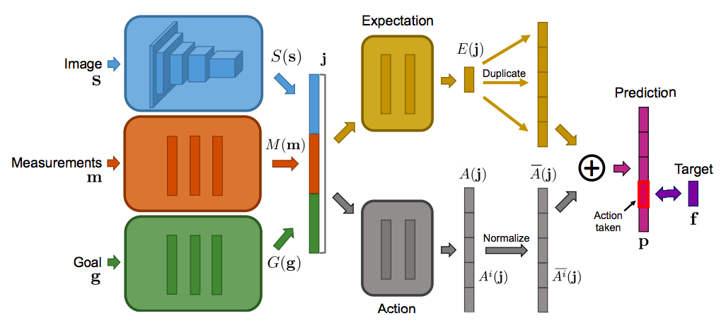
Notice that the model is split into 2 streams, the expectation stream \(E(j)\) and the Action stream \(A(j)\). The decision of using 2 separate streams is based on the dueling architecture introduced by DeepMind. Empirally, It usually leads to better performance empirically.

At training time, each transition through the environment produces a tuple <\(s\), \(a\), \(m\)>, where \(s\) represents the state (e.g. image pixels), \(a\) is the action taken, and \(m\) is the measurements. We then formulate our training target \(f\) using the measurements obtained at the specified temporal offsets \(\tau\) (i.e. \([1,2,4,8,16,32]\)):

We use the target to train our the neural network model with backpropagation. Mean squared error (MSE) is used as the loss function.

Hopefully by now you have a good understanding of DFP, how and why it works, and its significance. I have also implemented DFP in Keras on the VizDoom Health Gathering scenario. For those of you who want to dig deeper into the technical details, feel free to check out my implementation here.

VizDoom Health Gathering Environment

I implemented DFP on the Health Gathering environment provided by VizDoom. It is a 3D partially observable environment. The objective of the agent is to survive the longest time as possible. At each time step, the agent’s health decreases such that in order to live longer, it has to locate and pick up health packs scattered across different parts of the map. At the same time, the agent also needs to avoid running into poison jars which will take away health.

The environment provides health level as the only measurement. I augmented the measurement to also include number of health packs and poison jars picked up by the agent by inferring pick up events from the change in health level in successive time steps. Hence, the resulting measurement vector for each time step consists of 3 elements [Health, HealthPacks, Poison].

DFP Keras Implementation

First, let’s go through the neural network implementation. As discussed above, there are 3 input modules to the model. The perception module is the environment state, which is just screen pixels in our case. We use a 3 layer convolutional neural network as the feature extractor to transform jthe screen pixels into a vector of length 512.

# Perception Module
state_input = Input(shape=(input_shape))
perception_feat = Convolution2D(32, 8, 8, subsample=(4,4), activation='relu')(state_input)
perception_feat = Convolution2D(64, 4, 4, subsample=(2,2), activation='relu')(perception_feat)
perception_feat = Convolution2D(64, 3, 3, activation='relu')(perception_feat)
perception_feat = Flatten()(perception_feat)
perception_feat = Dense(512, activation='relu')(perception_feat)

A 3 layer fully connected network is used to parse the measurement module and goal module.

Measurement Module:

# Measurement Module
measurement_input = Input(shape=((measurement_size,)))
measurement_feat = Dense(128, activation='relu')(measurement_input)
measurement_feat = Dense(128, activation='relu')(measurement_feat)
measurement_feat = Dense(128, activation='relu')(measurement_feat)

Goal Module:

# Goal Module
goal_input = Input(shape=((goal_size,)))
goal_feat = Dense(128, activation='relu')(goal_input)
goal_feat = Dense(128, activation='relu')(goal_feat)
goal_feat = Dense(128, activation='relu')(goal_feat)

We concatenate the outputs of the 3 modules to form a joint representation for further processing.

concat_feat = merge([perception_feat, measurement_feat, goal_feat], mode='concat')

The model is then split into 2 streams, the expectation stream and the action stream. Their respective outputs are summed to form the model’s prediction.

expectation_stream = Dense(measurement_pred_size, activation='relu')(concat_feat)

prediction_list = []
for i in range(action_size):
    action_stream = Dense(measurement_pred_size, activation='relu')(concat_feat)
    prediction_list.append(merge([action_stream, expectation_stream], mode='sum'))

For our problem, measurement_size is 3 (i.e. [Health, HealthPacks, Poison]), num_timesteps is 6 (i.e. \([1,2,4,8,16,32]\)) and the action_size is 3 (i.e. Turn Left, Turn Right, Move Forward).

Last, we compile our model with ADAM as optimizer and mean squared error (mse) as the loss metric.

model = Model(input=[state_input, measurement_input, goal_input], output=prediction_list)
adam = Adam(lr=learning_rate)
model.compile(loss='mse',optimizer=adam)

Similar to other RL algorithms, most of the logic is contained in the update step. So let’s go through it. First we sample a minibatch of sample trajectories from the Experience Replay buffer and initialize the corresponding states, measurements, goal and targets variables:

state_input = np.zeros(((batch_size,) + self.state_size)) # Shape batch_size, img_rows, img_cols, 4
measurement_input = np.zeros((batch_size, self.measurement_size))
goal_input = np.tile(goal, (batch_size, 1))
f_action_target = np.zeros((batch_size, (self.measurement_size * len(self.timesteps))))
action = []

We then compute our target for the model, which is, as you recall, the differences of future and present measurements for the set of temporal offsets \([1,2,4,8,16,32]\). The target for each action is assigned to the f_action_target variable.

for i, idx in enumerate(rand_indices):
    future_measurements = []
    last_offset = 0
    done = False
    for j in range(self.timesteps[-1]+1):
        if not self.memory[idx+j][5]: # if episode is not finished
            if j in self.timesteps: # 1,2,4,8,16,32
                if not done:
                    future_measurements += list( (self.memory[idx+j][4] - self.memory[idx][4]) )
                    last_offset = j
                else:
                    future_measurements += list( (self.memory[idx+last_offset][4] - self.memory[idx][4]) )
        else:
            done = True
            if j in self.timesteps: # 1,2,4,8,16,32
                future_measurements += list( (self.memory[idx+last_offset][4] - self.memory[idx][4]) )
    f_action_target[i,:] = np.array(future_measurements)

We then go ahead and fill up the rest of the variables with the minibatch samples drawn from the experience replay. f_target is the “ground truth label” we assign to our model for training.

for i, idx in enumerate(rand_indices):
    state_input[i,:,:,:] = self.memory[idx][0]
    measurement_input[i,:] = self.memory[idx][4]
    action.append(self.memory[idx][1])

f_target = self.model.predict([state_input, measurement_input, goal_input]) # Shape [32x18,32x18,32x18]

for i in range(self.batch_size):
    f_target[action[i]][i,:] = f_action_target[i]

What we are left to do is to simply call the training routine provided by Keras to perform gradient descent update.

loss = self.model.train_on_batch([state_input, measurement_input, goal_input], f_target)

That’s it. I strongly encourage you to test out the code yourself. You can find it in this github page.

Experiments

Empirically, I found that the measurement and goal input modules to be not so useful and even slightly harmful to the performance, so I decided to exclude them from the inputs. So only the perception module is used as inputs to the model. The measurements are normalized and a goal vector \(g\) of \([1,1,-1]\) (i.e coefficients for [Health, HealthPacks, Poison] measurements) is used.

40,000 episodes of DFP is run on the Health Gathering scenario. Here is a video of DFP agent playing an episode.

For comparison sake, I also ran the same number of episodes using Double DQN (DDQN). A scalar reward of +1 is given to the agent when it picks up Health Packs, and a negative penalty of -100 for dying. Average survival time (moving average over 50 episodes) is used as the metric for performance. Below is the performance chart.

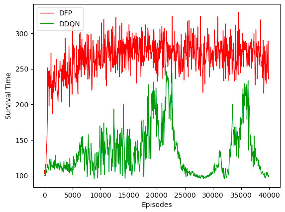
Notice that DFP converged very quickly in the first few hundred episodes. DDQN slowly caught up and its performance was almost on par with DFP at around episode 20,000, before it broke down completely. In contrast, DFP performance remained very stable throughout training.

As discussed above, DFP excels in environments where stream of rich and temporally dense multidimensional feedbacks is available. In traditional RL settings, transforming the feedbacks into a single dimension scalar reward might result in loss of useful information which would harm performance. In the ablation study carried out in the paper, the author pointed out that enrichment in measurements is the most important factor for the good performance of DFP.

Variation 1: Use Health as our only Measurement

Recall that in our implementation we have [Health, HealthPacks, Poison] as the measurements. HealthPacks and Poison are derivative measurements from Health (i.e. HealthPacks +1 when Health increases). What if right now we take away HealthPacks and Poison and use only [Health] as our measurement. Here is our result.

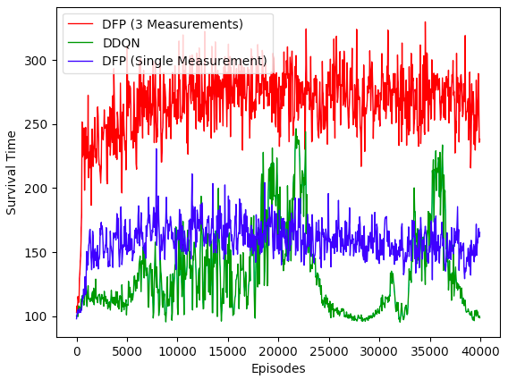
This is quite surprising and counterintuitive. The performance of DFP deteriorated by 50% if we just used [Health] as our only measurement (blue line), even though HealthPacks and Poisons are derived from the change in Health. I guess there is a beneficial effect by allowing the model to generate a richer set of predictions, similar to the way auxiliary tasks enhance performance of deep learning vision classifier. In fact, Google recently published a paper showing that addition of unsupervised auxiliary tasks leads to significant improvement over previous state of the art methods on Atari.

Variation 2: Change Goal to pick up Poison Jars

As discussed earlier, one of the best things about DFP is its capability to pursue different goals at inference time. To illustrate this, I used the trained model above and altered the goal vector \(g\) from \([1,1,-1]\) to \([0,0,1]\). The objective becomes

Which is to encourage the agent to pick actions that maximize the pick up of Poison Jars. Here is the video of the suicidal DFP agent playing an episode

Notice that the agent did not pick up any healthpacks but went directly for Poison instead!

Closing Thoughts

There are a couple of important takeaways from studying DFP.

1) If the environment provides us with a rich and temporally dense measurements signals, reformulating the RL problem to Supervised learning (e.g. DFP) may lead to better performance and accelerated training.

2) As shown from the experiments, more measurements almost certainly lead to better results. There is a beneficial effect by allowing the model to generate a richer set of predictions, similar to the way auxiliary tasks enhance performance of deep learning vision classifier.

3) The goal agnostic nature of DFP allows the agent to pursue complex goals at inference time. This lifts the limitation on learning and acting from a single objective by traditional RL methods, and is one way to achieve transfer learning and one shot learning for multiple tasks.

With that, thanks for reading the blogpost. I hope you that the post helps you better understand DFP and the benefits of reframing/augmenting RL with supervised learning. My Keras implementation of DFP can be found in my github. Feel free to use it for your own problem.

If you have any questions or thoughts feel free to leave a comment below.

You can also follow me on Twitter at @flyyufelix.